Marching Squares

June 27, 2013

Introduction

The marching squares algorithm is relatively simple, and it has a few unique applications, such as destructible terrain in video games and generating an outline of an image. It operates on a 2D grid whose cells' corners contain scalar values. The goal of marching squares is to classify cells using the values at their four respective corners. This algorithm is extremely fast, as well, which is always a good property to have!

Method

One use for marching squares is to create a 2D mesh, or contour, from a given grid. This example is rather simple, and it is easy to understand the idea behind marching squares. In other words, understanding the following implementation of marching squares is equivalent to understanding any other implementation of marching squares.

Here is the full algorithm in pseudocode:

marching_squares(grid):
  for all cells in grid:
      classify cell
  draw resulting mesh

Simple!

First, it is important to understand the exact details of the grid that is given as input because there is a subtle distinction to be made between the actual cells and their corners. Let's say, for example, the given grid has dimensions 2x2. This means that four cells need to be classified, and it means that there are exactly nine scalar values at all the corners of the grid. It's rather easy to confuse the values (corners) with the cells.

Here is an example of a possible 2x2 grid:

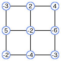
To classify a cell in the grid, create a bitmask representing the four corners of the cell. If you aren't familiar with the term "bitmask", don't worry. It isn't scary. A bitmask is just a series of 0s and 1s. In this case, the bitmask is four bits long, and each bit corresponds to a corner of the cell. There is one small problem with this method, though. The values are not necessarily 0s and 1s because they can be any number! To fix this, define a threshold for the values. For example:

if value < 0:
  value = 0
else:
  value = 1

Now that the four values must be either 0 or 1, the values in the grid are the following:

To create a bitmask for the cell in the top-right of the grid, we build a string of bits starting at the top-left corner of that cell and move clockwise around that cell's corners. The resulting bitmask is 1100, and that is the classification for this cell.

Notice, there are sixteen possible bitmasks, or combinations of 0s and 1s. Let's make it easy and think of each bitmask as an integer, where 0000 converts to 0 in base 10 and 1111 converts to 15 in base 10. 1100 in binary converts to 12 in base 10, so the cell we just dealt with has a classification of 12.

The only step left in creating the 2D mesh is to graphically represent the classification of each cell in the grid. Again, there are sixteen different classifications, so each case must be explicitly handled. It makes sense to define an image for each classification. One could imagine the following as a reasonable representation of the sixteen classifications to generate a 2D mesh:

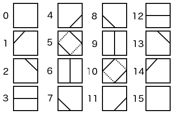
An interesting thing happens with cases 5 and 10. They are ambiguous, meaning either of the representations given in the diagram above are valid interpretations of the bitmask. In mathematical terms, they are called saddle points. Since they are ambiguous, they must be resolved somehow, and however they are resolved is highly dependent on the application. For this 2D mesh, it really doesn't matter. See if you can determine how I resolved the ambiguity in the demo below! (It should not be difficult.)

Finally, to generate and display the 2D mesh, the grid is drawn such that each cell is drawn by using the image corresponding to that cell's classification. The demo below implements the marching squares algorithm and generates a 2D mesh. You can change the values at the the corners of cells by clicking on them. The values simply toggle between 0 and 1.

Marching Squares Mesh Generator

Other Applications

Generating a 2D mesh is one of the simplest applications for the marching squares algorithm, but the concept remains the same no matter what the application is. If you read the Wikipedia article on marching squares, you will see that the 2D mesh application is sometimes called "isobanding". It gets the name from the use of the binary threshold on the values. One could imagine filtering the values into ternary or quaternary values to generate more interesting meshes.

Marching squares scales up to three dimensions, too. However, it takes on the clever name of "marching cubes". Again, the concept is exactly the same, except the bitmasks will be six bits long because a cube has six corners.

Of course, there are many other discussions about this algorithm all over the internet. Here are two particularly interesting ones: